First make a variable that shows production by land used
croptimeseries$production_byland=croptimeseries$`Production (million bushels)`/croptimeseries$`Planted area (million acres)`
Exponential Smoothing
Use the created variable to predict a exponential smoothing with a damping value of .9. (we will ignore .1 for this example)
Because R's ets() function is designed to automatically optimize and validate model parameters — and it will reject combinations (like AAN with phi = 0.1) that it determines are unstable or inappropriate for your data.
In contrast, Excel doesn’t optimize or reject your model. It simply applies the formula, even if it results in poor or unstable forecasts.
# Ensure your variable is a time series object# Replace the frequency and start values as neededts_data <-ts(croptimeseries$production_byland, frequency =1)# Exponential smoothing with damping value = 0.9model_damped_09 <-ets(ts_data, model ="AAN", damped =TRUE, phi =0.9)forecast_damped_09 <-forecast(model_damped_09)# Get fitted values (same length as original data)croptimeseries$fit_damped_09 <-as.numeric(fitted(model_damped_09))
Moving Average
Create a moving average using the interval of a decade.
Explanation
order = 10 — the window size (10 years)
# Apply 10-year (decade) moving averagecroptimeseries$ma_10yr <-ma(ts_data, order =10)
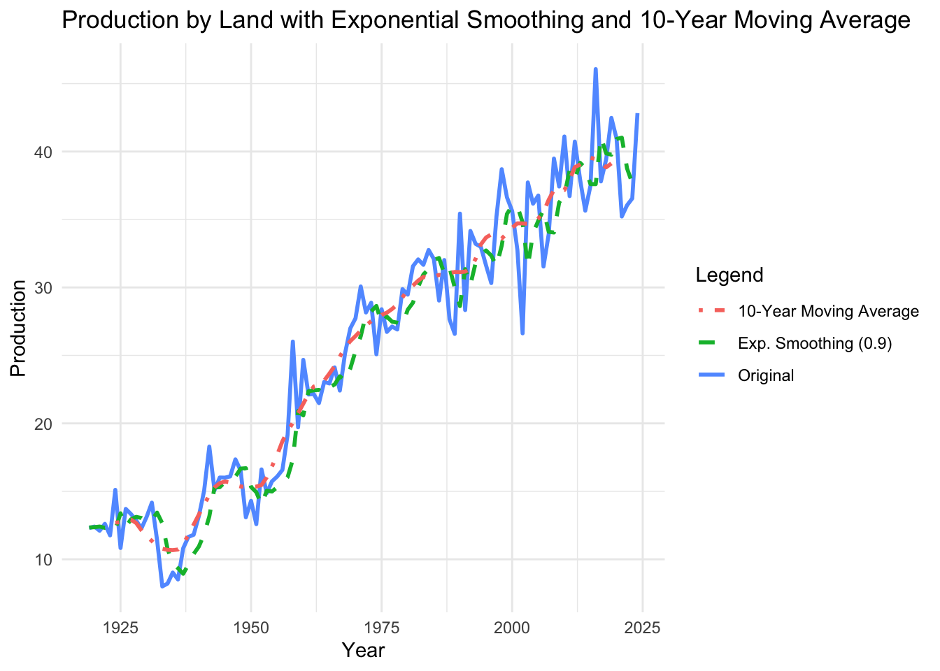
Line Graph
Create a line graph that including your production by land (1), the exponential smoothing (2) and the moving average (3)
ggplot(croptimeseries, aes(x = Year)) +# Make sure 'Year' exists and is correctgeom_line(aes(y = production_byland, color ="Original"), size =1) +geom_line(aes(y = fit_damped_09, color ="Exp. Smoothing (0.9)"), size =1, linetype ="dashed") +geom_line(aes(y = ma_10yr, color ="10-Year Moving Average"), size =1, linetype ="dotdash") +labs(title ="Production by Land with Exponential Smoothing and 10-Year Moving Average",x ="Year",y ="Production",color ="Legend") +theme_minimal()
Warning: Using `size` aesthetic for lines was deprecated in ggplot2 3.4.0.
ℹ Please use `linewidth` instead.
Warning: Removed 10 rows containing missing values or values outside the scale range
(`geom_line()`).
---title: "Time Series"author: "LoweMackenzie"date: 2024-10-20format: html: code-fold: false # Enables dropdown for code code-tools: true # (Optional) Adds buttons like "Show Code" code-summary: "Show code" # (Optional) Custom label for dropdown toc: true toc-location: left page-layout: fulleditor: visual---## # Times Series ExampleWe will use this page to cover the example we did in class.## LibrariesFirst load these libraries. *Remove hashtag before install.package to load library.*```{r}# Install the forecast package if not already installed#install.packages("forecast")# Load the packagelibrary(forecast)library(ggplot2)```## DataAnd the following data *Remember to switch the directory as this one is specific to my computer!*```{r}library(readxl)croptimeseries<-read_excel("/Users/ashleylowe/Desktop/SpreadsheetModeling429/2025/In-class/croptimeseries.xlsx")```## In - Class Example### Create Variable1. First make a variable that shows production by land used```{r} croptimeseries$production_byland=croptimeseries$`Production (million bushels)`/croptimeseries$`Planted area (million acres)```` ### Exponential Smoothing2. Use the created variable to predict a exponential smoothing with a damping value of .9. **(we will ignore .1 for this example)**Because **R\'s `ets()` function is designed to automatically optimize and validate model parameters** --- and it will **reject combinations** (like `AAN` with `phi = 0.1`) that it determines are **unstable or inappropriate** for your data.In contrast, **Excel doesn't optimize or reject your model**. It simply applies the formula, even if it results in poor or unstable forecasts.```{r}# Ensure your variable is a time series object# Replace the frequency and start values as neededts_data <-ts(croptimeseries$production_byland, frequency =1)# Exponential smoothing with damping value = 0.9model_damped_09 <-ets(ts_data, model ="AAN", damped =TRUE, phi =0.9)forecast_damped_09 <-forecast(model_damped_09)# Get fitted values (same length as original data)croptimeseries$fit_damped_09 <-as.numeric(fitted(model_damped_09))```### Moving Average3. Create a moving average using the interval of a decade. Explanation - `order = 10` --- the window size (10 years)```{r}# Apply 10-year (decade) moving averagecroptimeseries$ma_10yr <-ma(ts_data, order =10)```### Line Graph4. Create a line graph that including your production by land (1), the exponential smoothing (2) and the moving average (3)```{r}ggplot(croptimeseries, aes(x = Year)) +# Make sure 'Year' exists and is correctgeom_line(aes(y = production_byland, color ="Original"), size =1) +geom_line(aes(y = fit_damped_09, color ="Exp. Smoothing (0.9)"), size =1, linetype ="dashed") +geom_line(aes(y = ma_10yr, color ="10-Year Moving Average"), size =1, linetype ="dotdash") +labs(title ="Production by Land with Exponential Smoothing and 10-Year Moving Average",x ="Year",y ="Production",color ="Legend") +theme_minimal()```### MFE Calculation```{r}mean( croptimeseries$production_byland- croptimeseries$fit_damped_09, na.rm =TRUE)mean(croptimeseries$production_byland - croptimeseries$fit_damped_1 , na.rm =TRUE)mean( croptimeseries$production_byland - croptimeseries$ma_10yr , na.rm =TRUE)```